
Exploring genome annotation from Ensembl
Human genome annotation
You now know many ways of manipulating data inside R, and will also be familiar with some of the information stored in Ensembl. Let’s do some exercises using real data from Ensembl, specifically using gene annotation from the human genome. There are many ways to access these kinds of data, but I downloaded a GTF (General Transfer Format) file from Ensembl. They are available from the Downloads menu from the Ensembl FTP.

GTF files contain a lot of extra information we do not need right now, so I selected the most important bits and saved them as a regular table for loading into R. You can download the file we will be using here: Homo_sapiens.GRCh38.96.tab. Let me confess that to make our work easier Today, I removed most isoforms, only keeping the longest transcript for each gene.
Let us load the file into R and start exploring the data!
ensTab <- read.table("Homo_sapiens.GRCh38.96.tab", header=TRUE)As a reminder, it is always a good idea to have a quick check of the size of the data and a peak at its contents. For this we can check it’s dimensions and look at it’s head.
dim(ensTab)## [1] 283999 9head(ensTab)## chromosome start length strand type gene_id gene_name transcript_id transcript_biotype
## 1 1 17369 68 - transcript ENSG00000278267 MIR6859-1 ENST00000619216 miRNA
## 2 1 17369 68 - exon ENSG00000278267 MIR6859-1 ENST00000619216 miRNA
## 3 1 29554 1544 + transcript ENSG00000243485 MIR1302-2HG ENST00000473358 lincRNA
## 4 1 29554 486 + exon ENSG00000243485 MIR1302-2HG ENST00000473358 lincRNA
## 5 1 30564 104 + exon ENSG00000243485 MIR1302-2HG ENST00000473358 lincRNA
## 6 1 30976 122 + exon ENSG00000243485 MIR1302-2HG ENST00000473358 lincRNAThis is quite a big table, with 283999 rows! We really do NOT want to load up such a file in Excel! Let us look at the names of the columns again, to get a better idea of what is stored within.
colnames(ensTab)## [1] "chromosome" "start" "length" "strand" "type"
## [6] "gene_id" "gene_name" "transcript_id" "transcript_biotype"(there is also a function called rownames(), although in this case our table does not contain rownames)
That column type sounds interesting, let’s find out what values it has and how many of each:
table(ensTab$type)##
## exon transcript
## 239989 44010A more general and useful way of getting an overview of our data is to use the summary() function.
summary(ensTab)## chromosome start length strand type gene_id
## Length:283999 Min. : 3307 Min. : 1 Length:283999 Length:283999 Length:283999
## Class :character 1st Qu.: 31968289 1st Qu.: 101 Class :character Class :character Class :character
## Mode :character Median : 62510577 Median : 153 Mode :character Mode :character Mode :character
## Mean : 75595771 Mean : 5573
## 3rd Qu.:111896814 3rd Qu.: 371
## Max. :248936581 Max. :2471657
## gene_name transcript_id transcript_biotype
## Length:283999 Length:283999 Length:283999
## Class :character Class :character Class :character
## Mode :character Mode :character Mode :character
##
##
## So, this table contains all the annotated transcripts and their exons in the human genome. Not only protein_coding transcripts, but also lincRNAs, processed_pseudogenes, snRNA, etc. The chromosome, start position and strand is stored, as well as the length of each element. Ensembl gene ids and common name are also there. From the head() function, we can see that each row contains a distinct transcript OR exon, with the information we have just mentioned.
The following exercises are just a small set of questions that you can answer using R. Let’s first focus on the information regarding transcripts, by selecting and saving that portion of the table.
transTab <- ensTab[ensTab$type == "transcript",]

dim(transTab)
## [1] 44010 9head(transTab)## chromosome start length strand type gene_id gene_name transcript_id transcript_biotype
## 1 1 17369 68 - transcript ENSG00000278267 MIR6859-1 ENST00000619216 miRNA
## 3 1 29554 1544 + transcript ENSG00000243485 MIR1302-2HG ENST00000473358 lincRNA
## 7 1 30366 138 + transcript ENSG00000284332 MIR1302-2 ENST00000607096 miRNA
## 9 1 34554 1528 - transcript ENSG00000237613 FAM138A ENST00000417324 lincRNA
## 13 1 65419 6167 + transcript ENSG00000186092 OR4F5 ENST00000641515 protein_coding
## 17 1 92230 36988 - transcript ENSG00000238009 AL627309.1 ENST00000477740 lincRNAExercises
How many protein_coding transcripts are there in the human genome?
And how many miRNA (micro RNA) transcripts are there?
How about calculating the number of all the NON protein_coding transcripts?
Too easy? How many different ways can you think of to answer the above questions?
Let’s get all the lengths of the protein_coding transcripts. How about calculating the
meanand visualizing the distribution of the lengths as a histogram?Now that we have the code, let’s also look at the lengths of the miRNAs.
Now that we’re at it, what is the total number of bases covered by all the transcripts in the human genome?
If you answered the last question, perhaps you wondered just how much of the human genome is potentially transcribed. Perhaps the vast majority? You might have read somewhere about the dark matter of the genome or junk DNA, and how the majority of the human genome is not really coding. In any case, in order to compare the values we can calculate, we need to know the total size of the human genome. Do you know it? Fortunately Ensembl contains information for all the genomes it stores, including the human genome
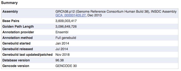
So, let’s store this number as a reference
gnmSize <- 3096649726Now, let’s go back to our answers to the previous exercises, and give them a bit more context.
Exercises
- What percent of the human genome is covered by protein_coding transcripts?
- What percent by miRNA transcripts?
- Better still, calculate the percent covered by protein_coding and also all the other NON protein_coding transcripts together. What percent is not covered by ANY transcript? How about drawing a
pie()with this information?
 - Does this result sound reasonable?
It’s very easy to make mistakes (remember the exons)
Until now, we have been ignoring the vast majority of the information in our table. That is, we have been looking only at the rows corresponding to transcripts, but have ignored the exons. What do we need the annotation of exons for?
At the very least, we know that transcripts can be spliced, and thus the transcribed region of the genome will actually be made up of exons and introns. Just how big are introns? We do not have to guess, it is better to use data to answer this question. But, these types of annotation file do not contain any explicit information about introns!
Perhaps looking at an example gene can help illustrate the information we do have:
ensTab[ensTab$gene_name == "NANOG",]## chromosome start length strand type gene_id gene_name transcript_id transcript_biotype
## 179842 12 7789402 9745 + transcript ENSG00000111704 NANOG ENST00000229307 protein_coding
## 179843 12 7789402 364 + exon ENSG00000111704 NANOG ENST00000229307 protein_coding
## 179844 12 7792950 263 + exon ENSG00000111704 NANOG ENST00000229307 protein_coding
## 179845 12 7794457 87 + exon ENSG00000111704 NANOG ENST00000229307 protein_coding
## 179846 12 7794679 4468 + exon ENSG00000111704 NANOG ENST00000229307 protein_codingNANOG is a key Transcription Factor that helps determine embryonic stem cell pluripotency (Wikipedia).
From our table, we can see that NANOG is encoded on chromosome 12, at position 7,789,402 on the + strand, and the transcript is 9,745 nt long. We can also see that if we add up all the exons (364 + 263 + 87 + 4468) they occupy 5,182 nt. So, how long are the introns for this gene?
Now that you’ve seen how easy it is, let’s tackle the big problem:
- What percent of the human genome is covered by exons, and what percent is covered by introns? Can you modify your previous
pie()to represent this?

Now that you’ve made a script to perform this analysis, how easy is it do adapt it for new data in the same format?
You can download the corresponding file for other organisms here: folder
Final Exercise
- Download the four tab files from the previous folder.
- Prepare a script that will cycle through each file and process them according to this pratical.
- At the end the script should produce a single PDF file with a pie for each species.